library(rgbif)
library(tidyverse)
library(data.table)
library(maps)
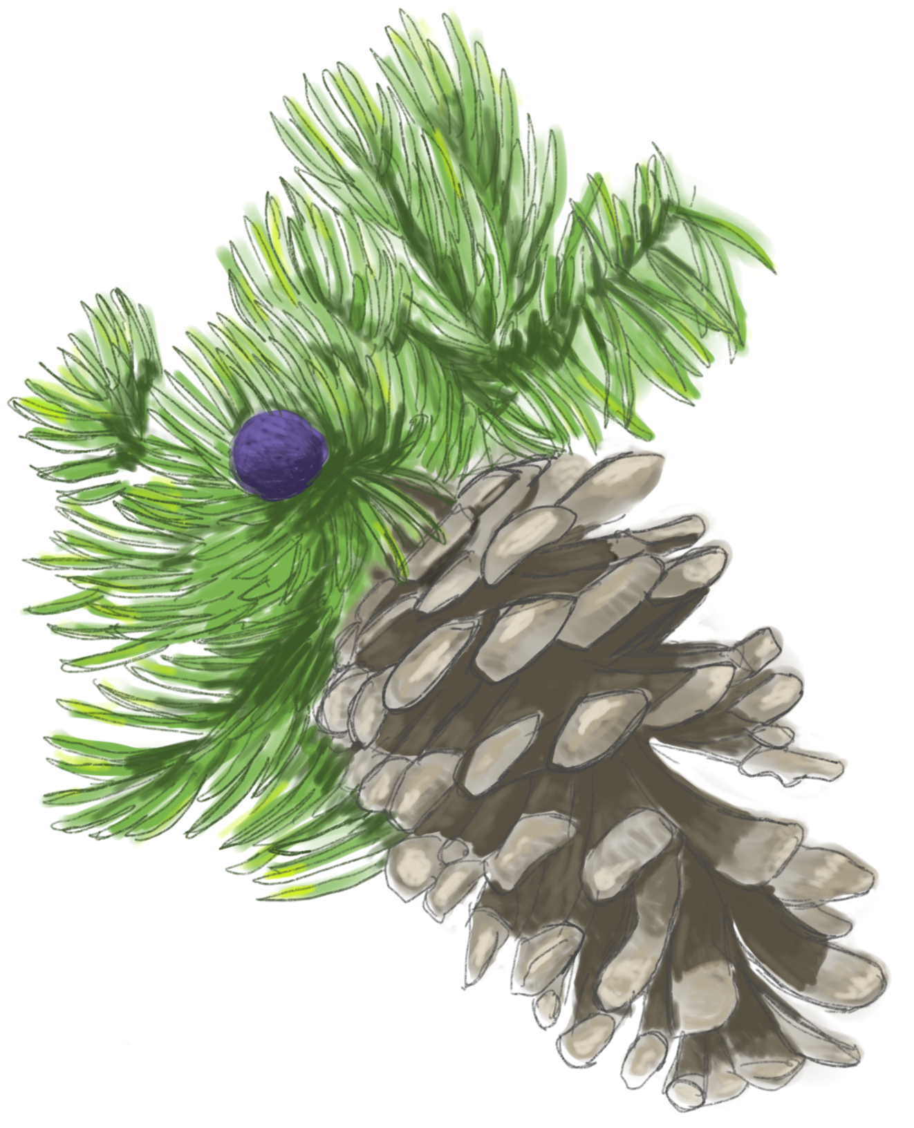
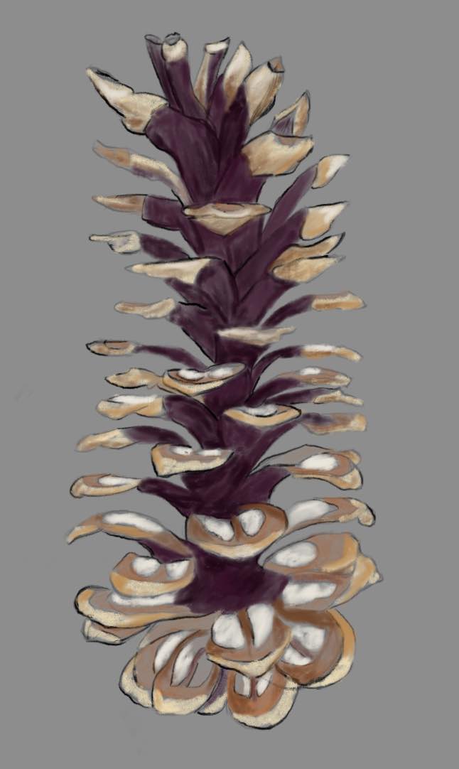
Continuing to check off the conifer species that occur in the Miracle Mile so I can make a visit and try to ID all of them. Last summer I found some Foxtail Pine (Pinus balfouriana) and (Pinus monticola) near Mount Eddy in the Klammath Range (among others).
Load the libraries.
Load the data.
ski_data <- read.csv("~/DATA/data/SkiTouring.csv")
TrailRun1 <- read.csv("~/DATA/data/TrailRun_FoxtailPine.csv")
Make a quick plot using the latitude and longitude coordinates and color by the date of the tour.
run1 <- ggplot(TrailRun1, aes(x = position_long, y = position_lat)) +
                    coord_quickmap() + geom_point()
run1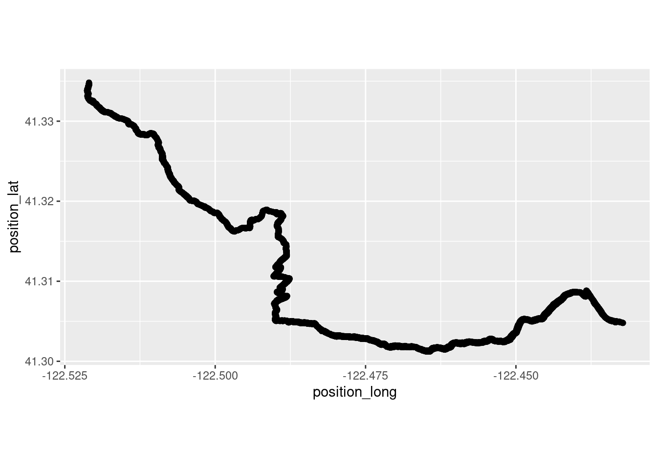
Make a general area polygon for GBIF and query the database to see if there are public observations of our two species of interest in the general region I ran in.
norcal_geometry <- paste('POLYGON((-122.6 41.35, -122.35 41.35, -122.35 41.25, -122.4 41.25, -122.6 41.25, -122.6 41.35))')

mm_species <- c("pinus balfouriana", "pinus monticola")

foxtail_data <- occ_data(scientificName = mm_species, hasCoordinate = TRUE, limit = 10000,
                   geometry = norcal_geometry)

foxtail_coords <- foxtail_data$data[ , c("decimalLongitude", "decimalLatitude",
 "individualCount", "occurrenceStatus", "coordinateUncertaintyInMeters",
  "institutionCode", "references")]

mm_all <- occ_data(scientificName = mm_species, hasCoordinate = TRUE, limit = 10000,
                   geometry = norcal_geometry)
mm_species_coords_list <- vector("list", length(mm_species))
names(mm_species_coords_list) <- mm_species
head(mm_species_coords_list)
$`pinus balfouriana`
NULL
$`pinus monticola`
NULLLoop through and make a dataframe from the lists.
for (x in mm_species) {
  coords <- mm_all[[x]]$data[ , c("decimalLongitude", "decimalLatitude", "occurrenceStatus", "coordinateUncertaintyInMeters", "institutionCode", "references")]
  mm_species_coords_list[[x]] <- data.frame(species = x, coords)
}

tree_df <- rbindlist(mm_species_coords_list, fill = T)
Just take a quick look at the raw observations plotted by latitude and longitude. Plot the species on the California map to see the limited polygon sampled.
maps::map(database = "state", region = "california")
points(tree_df[ , c("decimalLongitude", "decimalLatitude")], pch = ".", col = "blue", cex = 3)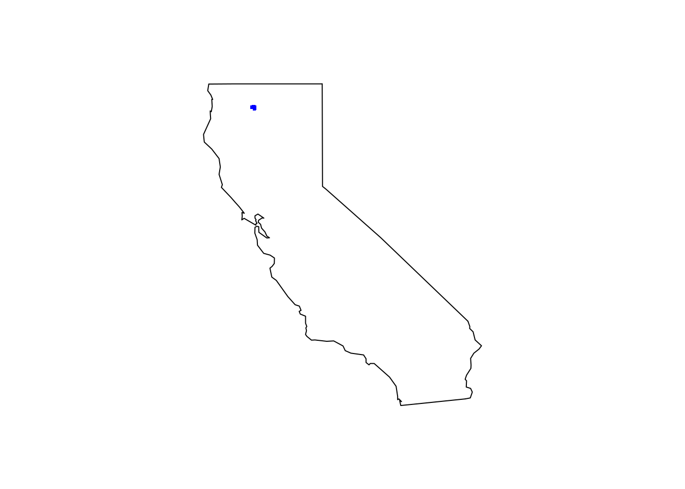
Plot all of the species using ggplot for the zoomed in area.
run_plot1  <- ggplot(tree_df, aes(x=decimalLongitude, y = decimalLatitude, color = species)) +
                             geom_point() + labs(color = "Species", title = "MM Zone")
run_plot1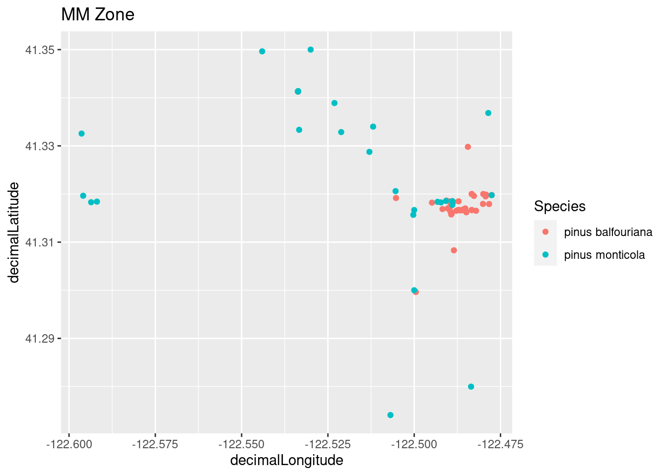
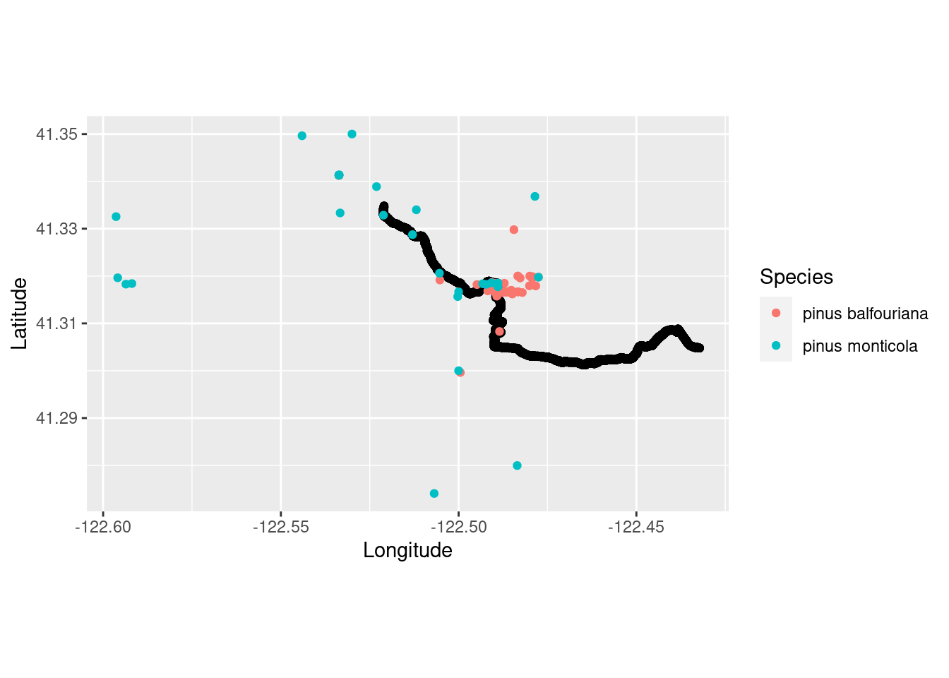
Combine trail running and species occurrence observations.
run_plot2 <- ggplot() +
          coord_quickmap() +
          geom_point(data = TrailRun1, aes(x = position_long, y = position_lat), color = 'black') +
          geom_point(data=tree_df, aes(x = decimalLongitude, y = decimalLatitude, color = factor(species))) +
          xlab("Longitude") + ylab("Latitude") + labs(color='Species')
run_plot2