Cody Markelz - Sugar Pine (Pinus lambertiana)

Another species found! I am attempting to ID all the conifer species that occur in the Miracle Mile while out on runs so I can make a visit to the Miracle Mile and ID all of them in one go.

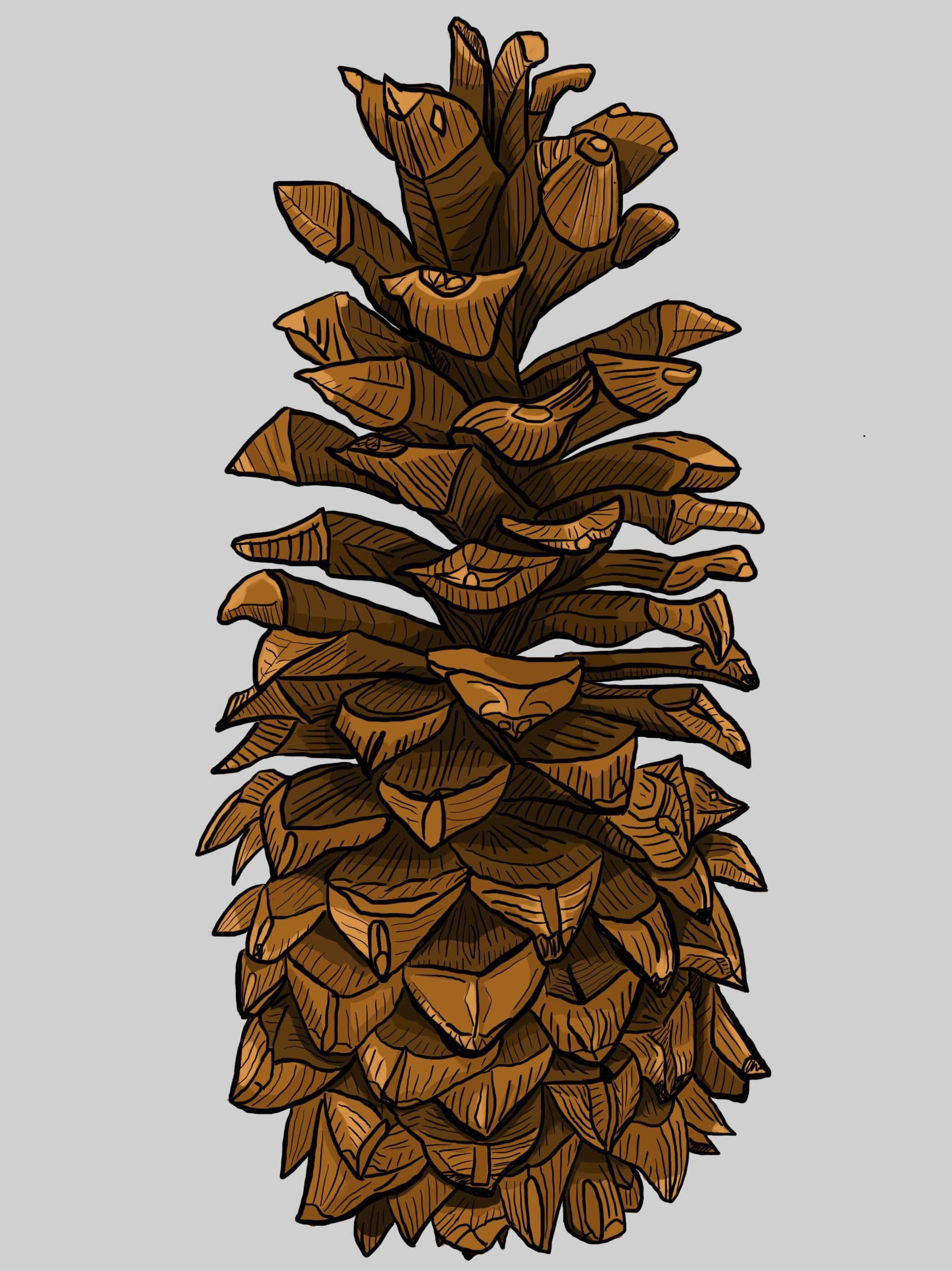
These sugar pine cones are huge! I have a few in my pinecone collection that are greater than 35 cm! Sugar pines (Pinus lambertiana) are fairly common species and I see them on trail runs often. For this post I first pulled the observations from GBIF, plotted them, and then looked where I had recently ran that would overlap with the species observation data. In this case, it was on a section of the Pacific Crest Trail (PCT) that I did an out and back run on.

library(rgbif)
library(tidyverse)
library(data.table)
library(maps)

Subset our search to only Northern California

mm_geometry <- paste('POLYGON((-124.4323 42.0021, -121.5045 42.0021, -121.5045 40.194, -124.4323 40.194, -124.4323 42.0021))')

Pull in the publicly available data and make a few quick plots.

pinus_lambertiana_NC <- occ_data(scientificName = "Pinus lambertiana", hasCoordinate = TRUE, limit = 10000,
                     geometry = mm_geometry )
head(pinus_lambertiana_NC)

$meta
$meta$offset
[1] 300

$meta$limit
[1] 2

$meta$endOfRecords
[1] TRUE

$meta$count
[1] 302


$data
# A tibble: 302 × 120
   key    scien…¹ decim…² decim…³ issues datas…⁴ publi…⁵ insta…⁶ publi…⁷ proto…⁸
   <chr>  <chr>     <dbl>   <dbl> <chr>  <chr>   <chr>   <chr>   <chr>   <chr>  
 1 40463… Pinus …    41.3   -122. cdc,c… 50c950… 28eb1a… 997448… US      DWC_AR…
 2 40463… Pinus …    41.3   -122. cdc,c… 50c950… 28eb1a… 997448… US      DWC_AR…
 3 34993… Pinus …    41.9   -124. cdc    50c950… 28eb1a… 997448… US      DWC_AR…
 4 37057… Pinus …    41.5   -124. cdc,c… 50c950… 28eb1a… 997448… US      DWC_AR…
 5 37053… Pinus …    41.2   -122. cdc,c… 50c950… 28eb1a… 997448… US      DWC_AR…
 6 37472… Pinus …    40.9   -124. cdc    50c950… 28eb1a… 997448… US      DWC_AR…
 7 37598… Pinus …    41.8   -124. cdc,c… 50c950… 28eb1a… 997448… US      DWC_AR…
 8 39613… Pinus …    40.4   -123. cdc,c… 50c950… 28eb1a… 997448… US      DWC_AR…
 9 37642… Pinus …    41.9   -124. cdc,c… 50c950… 28eb1a… 997448… US      DWC_AR…
10 37603… Pinus …    41.9   -124. cdc,c… 50c950… 28eb1a… 997448… US      DWC_AR…
# … with 292 more rows, 110 more variables: lastCrawled <chr>,
#   lastParsed <chr>, crawlId <int>, hostingOrganizationKey <chr>,
#   basisOfRecord <chr>, occurrenceStatus <chr>, taxonKey <int>,
#   kingdomKey <int>, phylumKey <int>, classKey <int>, orderKey <int>,
#   familyKey <int>, genusKey <int>, speciesKey <int>, acceptedTaxonKey <int>,
#   acceptedScientificName <chr>, kingdom <chr>, phylum <chr>, order <chr>,
#   family <chr>, genus <chr>, species <chr>, genericName <chr>, …

pinus_lambertiana_coords <- pinus_lambertiana_NC$data[ , c("decimalLongitude", "decimalLatitude", "occurrenceStatus", "coordinateUncertaintyInMeters", "institutionCode", "references")]

maps::map(database = "state", region = "california")
points(pinus_lambertiana_coords[ , c("decimalLongitude", "decimalLatitude")], pch = ".", col = "red", cex = 3)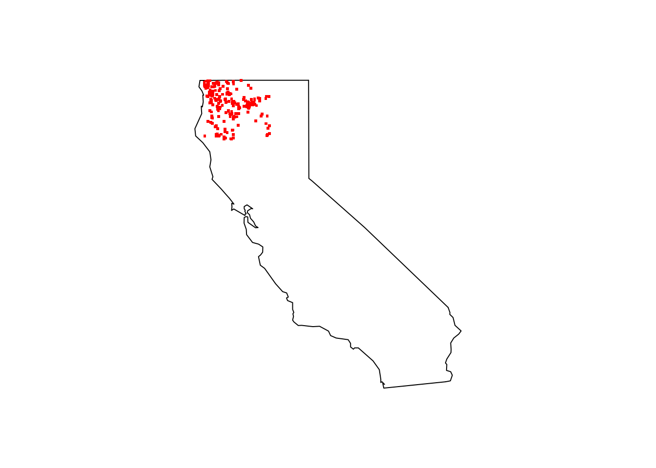

Pull in my run data.

TrailRun1  <- read.csv("~/DATA/data/TrailRun_SugarPine.csv")

Make a quick plot.

TrailRun_plot <- ggplot(TrailRun1, aes(x = position_long, y = position_lat)) +
                    coord_quickmap() + geom_point() +
                    xlab("Longitude") + ylab("Latitude")
TrailRun_plot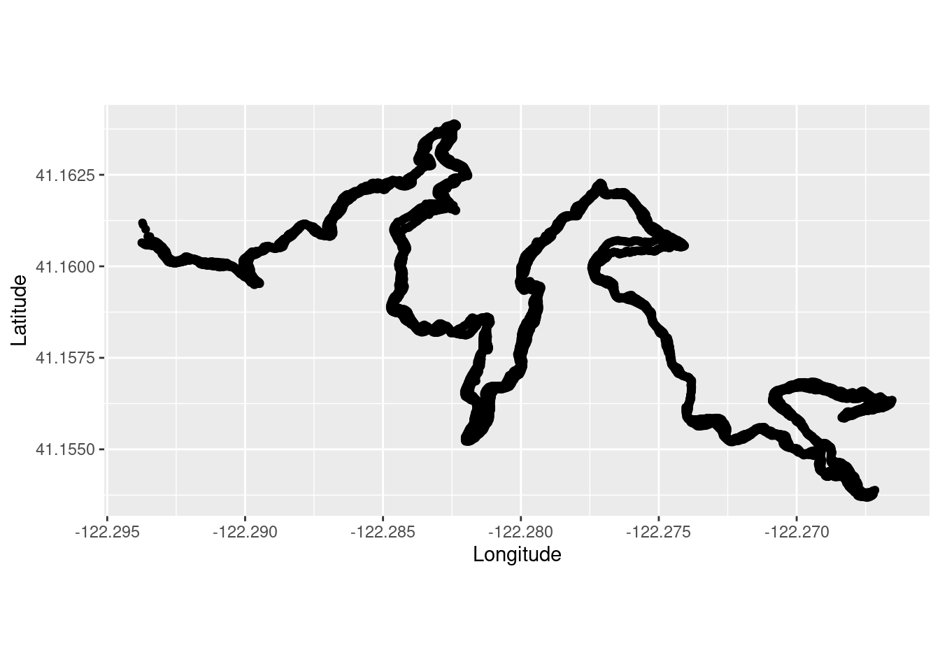

Subset the larger California dataset to only include a zoomed in portion where I ran based on the maximum and minimum coordinates from the run plot above.

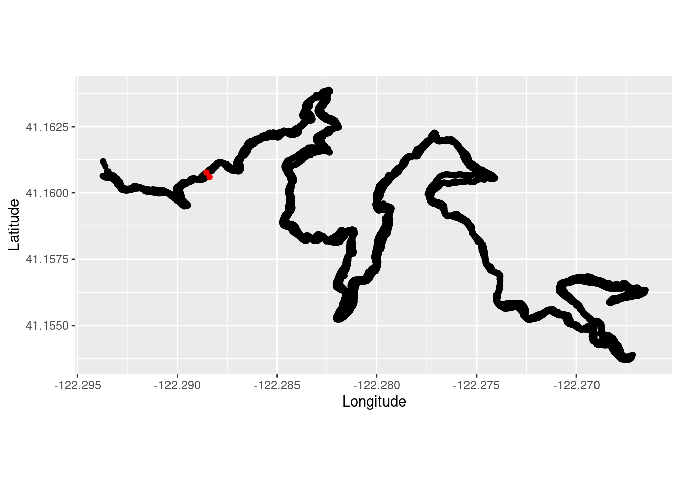
pinus_lamb_coords_sub <- subset(pinus_lambertiana_coords, decimalLatitude > 41.1525 & decimalLatitude < 41.1650 & decimalLongitude > -122.295 & decimalLongitude < -122.265 )

Overlay the plots!

TrailRun_plot2 <- ggplot() +
          coord_quickmap() +
          geom_point(data = TrailRun1, aes(x = position_long, y = position_lat), color = 'black') +
          geom_point(data=pinus_lamb_coords_sub, aes(x = decimalLongitude, y = decimalLatitude), color = 'red') +
          xlab("Longitude") + ylab("Latitude")
TrailRun_plot2