Cody Markelz - Bay Area Insects

I am working on a project using data collected at some of the UC Reserves. I needed to see what observations of insects were available in GBIF.

I found this drawing tool for bounding boxes. Make sure to export it as OGC WKT and then you can create a POLYGON to use as your query area.

reserve_geometry <- paste('POLYGON((-121.383275382 35.7567710044, -121.9875234289 36.3607073262, -122.525853507 37.2841110386, -123.1520742101 38.0753438834, -123.7123769445 38.8153202525, -123.8332265539 39.0972469563, -123.4596913976 39.2930774901, -122.0644277258 39.2250244313, -121.7568105383 38.0320888877, -121.4052480383 37.2578829342, -121.119603507 36.7402099684, -120.9987538976 36.1303379589, -121.383275382 35.7567710044))')

Load the libraries.

library(rgbif)
library(tidyverse)
library(maps)

Query the greater Bay Area for insects using the classKey for Insecta using the above geometry. Make a new dataframe with only the data from the query for plotting and data manipulation.

insect <- occ_data(classKey = 216, hasCoordinate = TRUE, limit = 1000, geometry = reserve_geometry)
insect_coords <- insect$data
head(insect_coords)

# A tibble: 6 × 78
  key     scien…¹ decim…² decim…³ issues datas…⁴ publi…⁵ insta…⁶ publi…⁷ proto…⁸
  <chr>   <chr>     <dbl>   <dbl> <chr>  <chr>   <chr>   <chr>   <chr>   <chr>  
1 401151… Dishol…    37.5   -122. cdc,c… 50c950… 28eb1a… 997448… US      DWC_AR…
2 401150… Dishol…    37.5   -122. cdc,c… 50c950… 28eb1a… 997448… US      DWC_AR…
3 401170… Forfic…    37.5   -122. cdc,c… 50c950… 28eb1a… 997448… US      DWC_AR…
4 401164… Danaus…    37.5   -122. cdc,c… 50c950… 28eb1a… 997448… US      DWC_AR…
5 401182… Aphis …    37.3   -122. cdc,c… 50c950… 28eb1a… 997448… US      DWC_AR…
6 401189… Vaness…    37.0   -122. cdc    50c950… 28eb1a… 997448… US      DWC_AR…
# … with 68 more variables: lastCrawled <chr>, lastParsed <chr>, crawlId <int>,
#   hostingOrganizationKey <chr>, basisOfRecord <chr>, occurrenceStatus <chr>,
#   taxonKey <int>, kingdomKey <int>, phylumKey <int>, classKey <int>,
#   orderKey <int>, familyKey <int>, genusKey <int>, speciesKey <int>,
#   acceptedTaxonKey <int>, acceptedScientificName <chr>, kingdom <chr>,
#   phylum <chr>, order <chr>, family <chr>, genus <chr>, species <chr>,
#   genericName <chr>, specificEpithet <chr>, taxonRank <chr>, …

Visualize the data for the state of California.

maps::map(database = "state", region = "california")
points(insect_coords[ , c("decimalLongitude", "decimalLatitude")], pch = ".", col = "blue", cex = 3)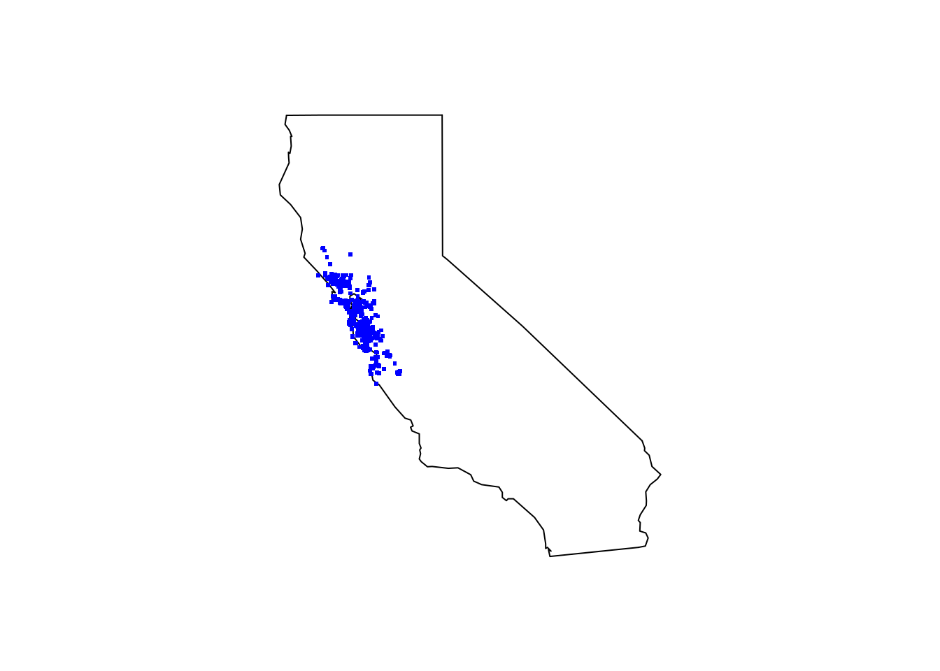

Randomly subset the coordinates dataframe and plot species by color. If you have a large screen, you can make a larger plotting window with many more species than 25.

set.seed(25344)
insect_coords_25 <- sample_n(insect_coords, 25)
species_plot1  <- ggplot(insect_coords_25, aes(x=decimalLongitude, y = decimalLatitude, color =acceptedScientificName)) +
       geom_point() + labs(x = "Longitude", y = "Latitude", color = "Species", title = "Bay Area Insect Distributions")
species_plot1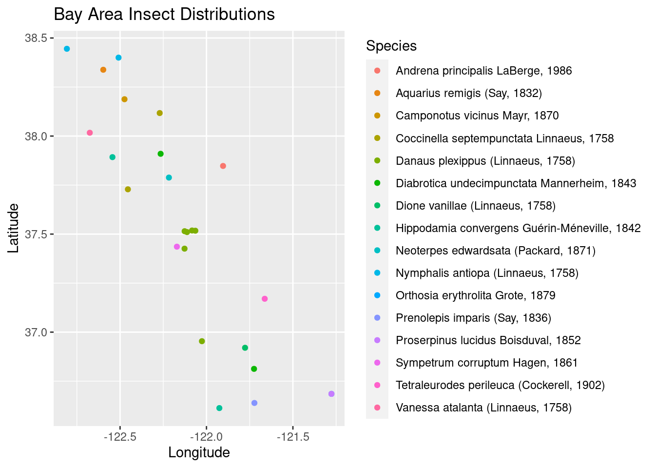

ggsave("~/DATA/images/bay_area_insects.png")