library(tidyverse)
library(rgbif)
library(gpx)
Spring is in full swing in the higher elevations around Mount Shasta and the surrounding ranges. I am always struck by the large patches of Cobra Lilies that grow along nutrient poor seeps in alpine meadows. I nearly always stop to take some photos and take in all the cool colors and shapes when out on training runs or hikes. I have made many observations of these over the past few years, but here is a quick post to pull out observations from GBIF.
Load the libraries.
Make the large Northern California polygon to look for observations in GBIF.
norcal_geometry <- paste('POLYGON((-124.4323 42.0021, -121.5045 42.0021, -121.5045 40.194, -124.4323 40.194, -124.4323 42.0021))')

cobra_lily <- occ_data(scientificName = "darlingtonia californica", hasCoordinate = TRUE, limit = 1000,
                   geometry = norcal_geometry)
head(cobra_lily)
$meta
$meta$offset
[1] 900
$meta$limit
[1] 100
$meta$endOfRecords
[1] FALSE
$meta$count
[1] 1582
$data
# A tibble: 1,000 × 128
key scien…¹ decim…² decim…³ issues datas…⁴ publi…⁵ insta…⁶ hosti…⁷ publi…⁸
<chr> <chr> <dbl> <dbl> <chr> <chr> <chr> <chr> <chr> <chr>
1 45123… Darlin… 41.7 -124. cdc,c… 50c950… 28eb1a… 997448… 28eb1a… US
2 45163… Darlin… 41.9 -124. cdc,c… 50c950… 28eb1a… 997448… 28eb1a… US
3 45191… Darlin… 41.9 -124. cdc,c… 50c950… 28eb1a… 997448… 28eb1a… US
4 45253… Darlin… 41.9 -124. cdc,c… 50c950… 28eb1a… 997448… 28eb1a… US
5 45280… Darlin… 41.7 -124. cdc,c… 50c950… 28eb1a… 997448… 28eb1a… US
6 40286… Darlin… 41.9 -124. cdc,c… 50c950… 28eb1a… 997448… 28eb1a… US
7 40347… Darlin… 40.7 -124. cdc,c… 50c950… 28eb1a… 997448… 28eb1a… US
8 40394… Darlin… 41.6 -124. cdc,c… 50c950… 28eb1a… 997448… 28eb1a… US
9 41655… Darlin… 41.8 -124. cdc,c… 50c950… 28eb1a… 997448… 28eb1a… US
10 40629… Darlin… 41.9 -124. cdc,c… 50c950… 28eb1a… 997448… 28eb1a… US
# … with 990 more rows, 118 more variables: protocol <chr>, lastCrawled <chr>,
# lastParsed <chr>, crawlId <int>, basisOfRecord <chr>,
# occurrenceStatus <chr>, taxonKey <int>, kingdomKey <int>, phylumKey <int>,
# classKey <int>, orderKey <int>, familyKey <int>, genusKey <int>,
# speciesKey <int>, acceptedTaxonKey <int>, acceptedScientificName <chr>,
# kingdom <chr>, phylum <chr>, order <chr>, family <chr>, genus <chr>,
# species <chr>, genericName <chr>, specificEpithet <chr>, taxonRank <chr>, …Quick map of observations.
cobra_lily_coords <- cobra_lily$data[ , c("decimalLongitude", "decimalLatitude", "occurrenceStatus", "coordinateUncertaintyInMeters", "institutionCode", "references")]

maps::map(database = "state", region = "california")
points(cobra_lily_coords[ , c("decimalLongitude", "decimalLatitude")], pch = ".", col = "red", cex = 3)
Pull in my run data using the gpx R library and subset the route to make plotting easier.
run <-  read_gpx('~/DATA/data/cobra_lily_run.gpx')
TrailRun1 <- as.data.frame(run$routes)
Make a quick run plot.
TrailRun_plot <- ggplot() +
          geom_point(data = TrailRun1, aes(x = Longitude, y = Latitude), color = 'black') +
          xlab("Longitude") + ylab("Latitude")
TrailRun_plot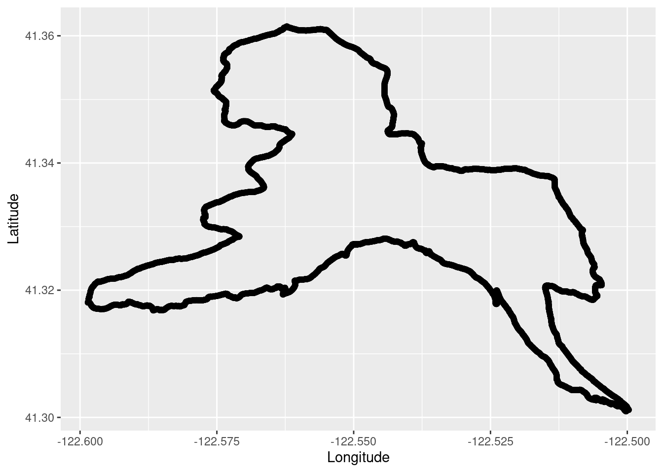
Subset the larger California dataset to only include a zoomed in portion where I ran based on the maximum and minimum coordinates from the run plot above.
cobra_lily_coords_sub <- subset(cobra_lily_coords, decimalLatitude > 41.3 & decimalLatitude < 41.365 & decimalLongitude > -122.6 & decimalLongitude < -122.5 )Overlay the plots and add a triangle for the seep where I observed some Cobra Lilies next to the trail.
TrailRun_plot2 <- ggplot() +
          coord_quickmap() +
          geom_point(data = TrailRun1, aes(x = Longitude, y = Latitude), color = 'black') +
          geom_point(data=cobra_lily_coords_sub, aes(x = decimalLongitude, y = decimalLatitude), color = 'red') +
          geom_point(aes(x = -122.55, y = 41.325), pch=25, size= 12, colour="purple") +
          xlab("Longitude") + ylab("Latitude")
TrailRun_plot2
In a follow-up post we will import some additional environmental data to make a multi-layered map.