library(tidyverse)
library(gpx)
library(rayshader)
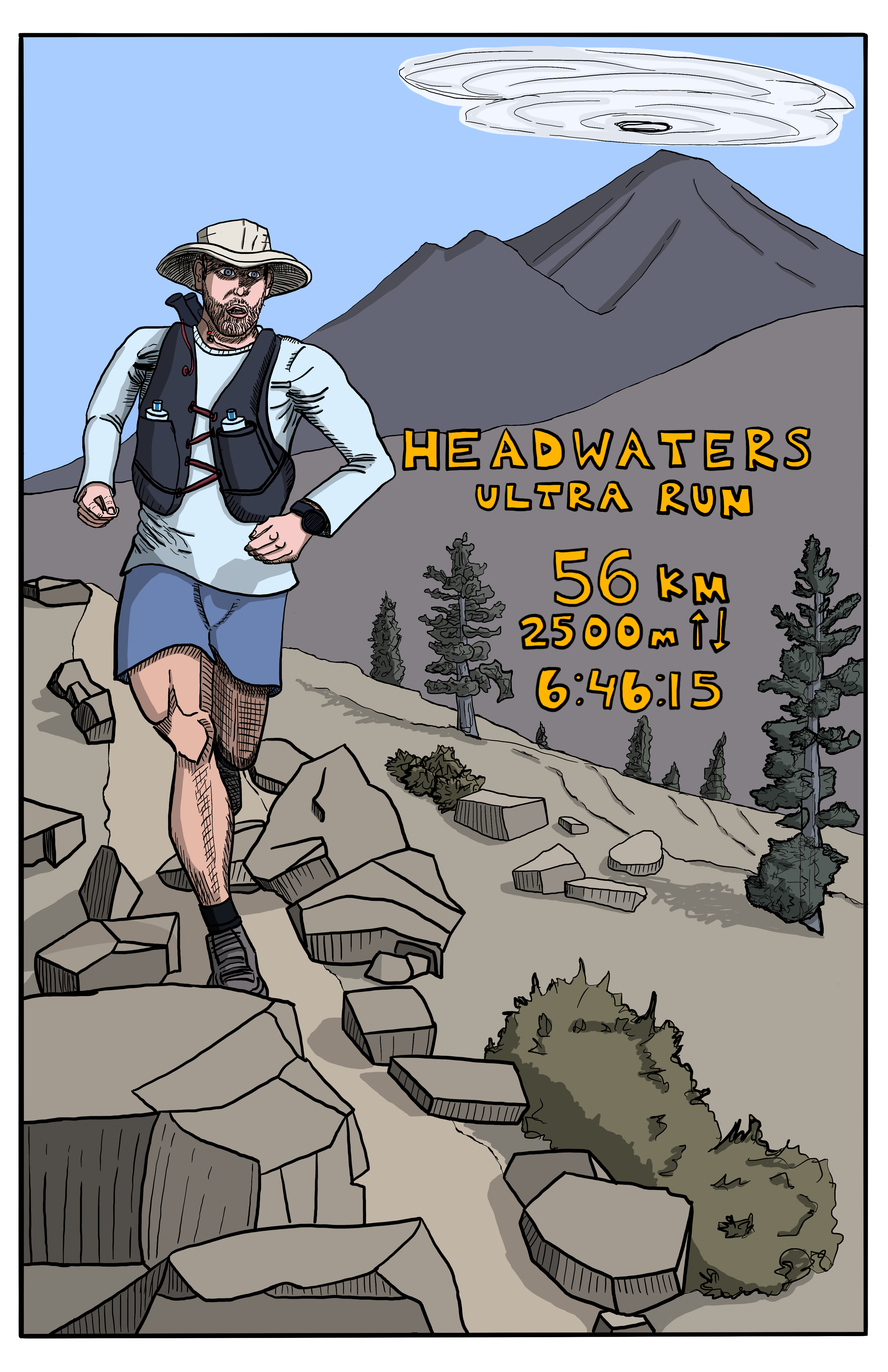
Last month I ran the Headwaters Ultra here in Mount Shasta, CA. The race starts at Lake Siskiyou, heads up the steep trails on Rainbow Ridge and then heads over into the Eddy Range in the Klamath Mountains. The course meets up with the Sisson-Callahan Trail to go up and over the saddle (~8000 ft) just below the summit trail to the top of Mount Eddy (9,037 ft; 2,754 m). After the last aid station at Deadfall Meadows, the course goes back up and over the saddle followed by 12 miles of fast, quad-busting descent all the way down the Sisson-Callahan trial. It was really fun overall. It rained and snowed the night before, so the race went through a few inches of fresh snow at the higher elevations above ~6500 ft. The moody dark clouds at higher elevations were interrupted by moments of bright sunshine poking through reflecting off the snow and illuminating the Foxtail Pine Grove. I finished the race 8th overall with a time of 6:44:15. A great day out!
Take a quick look at some of the course data collected by my exercise watch.
Load the libraries.
Pull in my run data using the gpx R library and subset the route to make plotting easier. Add a Time column for seconds elapsed for plotting purposes.
run <-  read_gpx('~/DATA/data/headwaters-2022-06-18.gpx')
summary(run)
Length Class Mode
routes 1 -none- list
tracks 1 -none- list
waypoints 1 -none- listTrailRun1 <- as.data.frame(run$routes)
TrailRun1$Time <- as.numeric(row.names(TrailRun1))Quick plot.
TR_p1 <- ggplot() +
          geom_point(data = TrailRun1, aes(x = Longitude, y = Latitude), color = 'black', size = 2) +
          xlab("Longitude") + ylab("Latitude")
TR_p1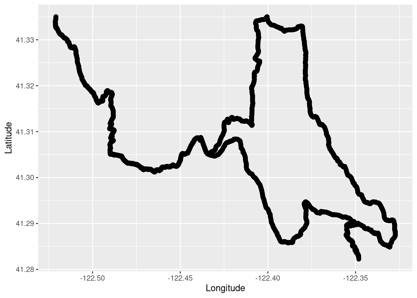
Take a look at the elevation profile in meters.
TR_p2 <- ggplot() +
          geom_line(data = TrailRun1, aes(x = Time, y = Elevation), color = 'black', size = 2) +
          xlab("Time (seconds)") + ylab("Elevation (m)")
TR_p2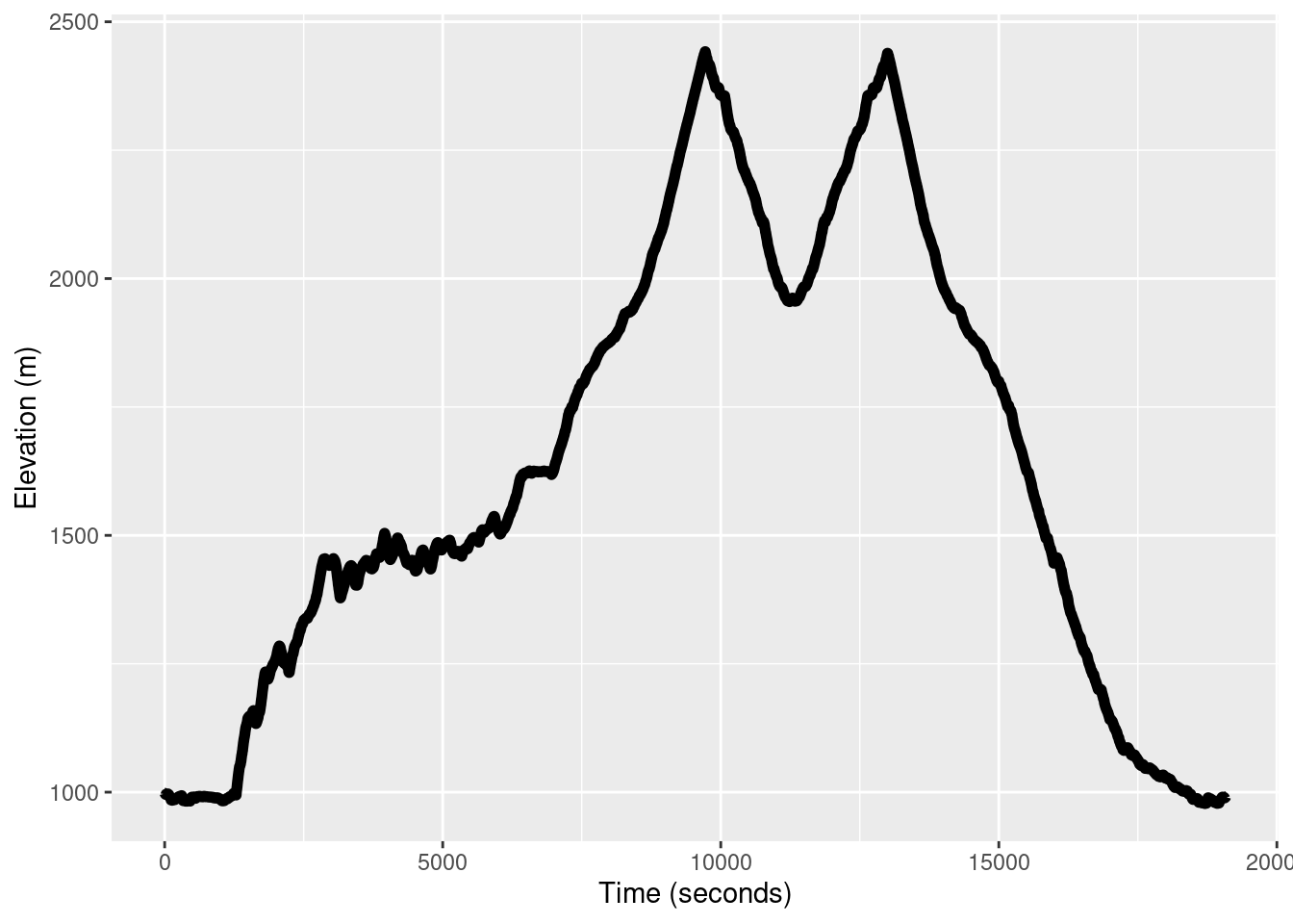
Make a new factor column to see what parts of the race had snow on them.
TrailRun1$snow <-  as.factor(if_else(TrailRun1$Elevation > 1980, "Yes", "No"))
TR_p3 <- ggplot() +
          geom_line(data = TrailRun1, aes(x = Time, y = Elevation, color = snow), size = 2) +
          xlab("Time (seconds)") + ylab("Elevation (m)")
TR_p3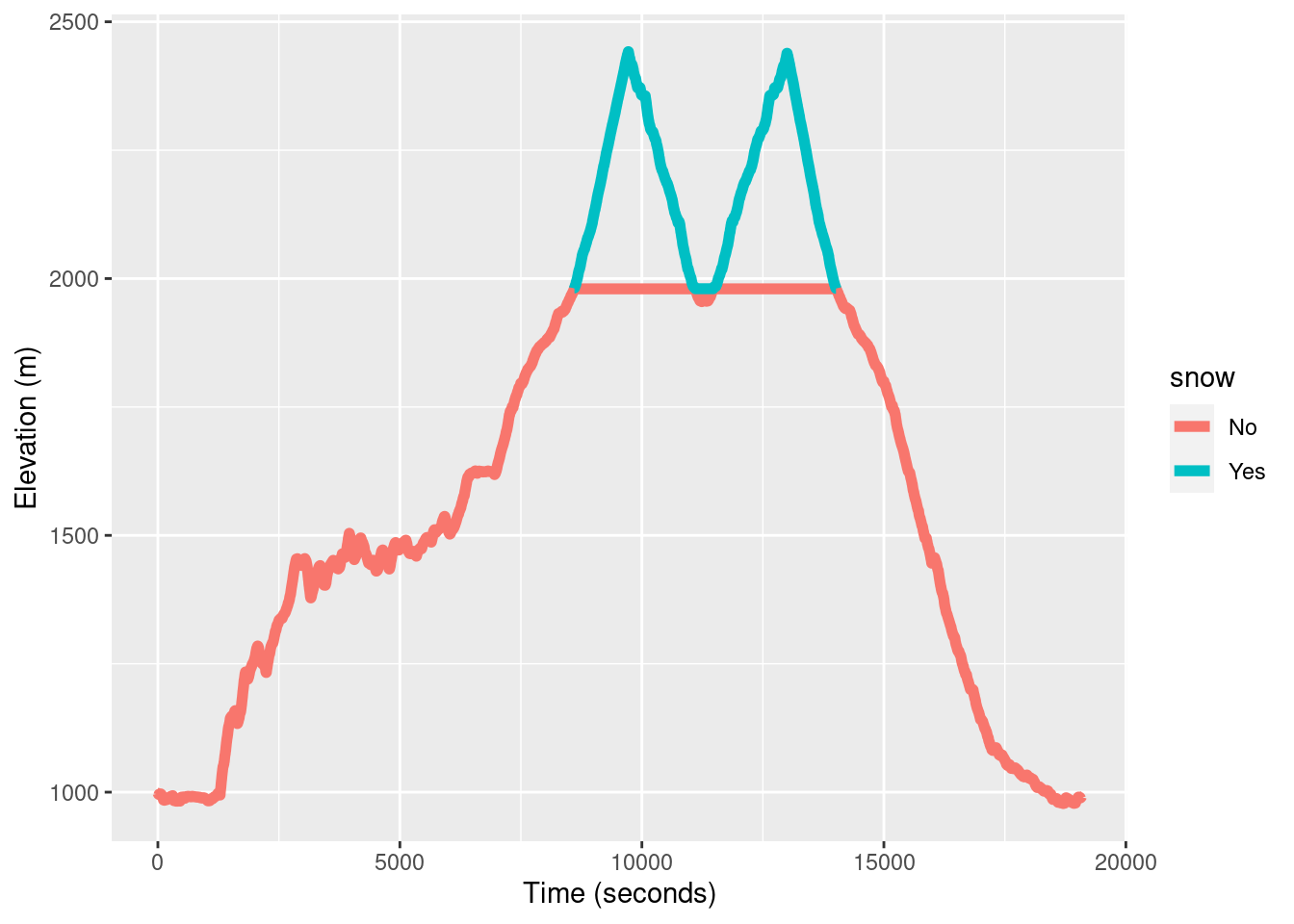
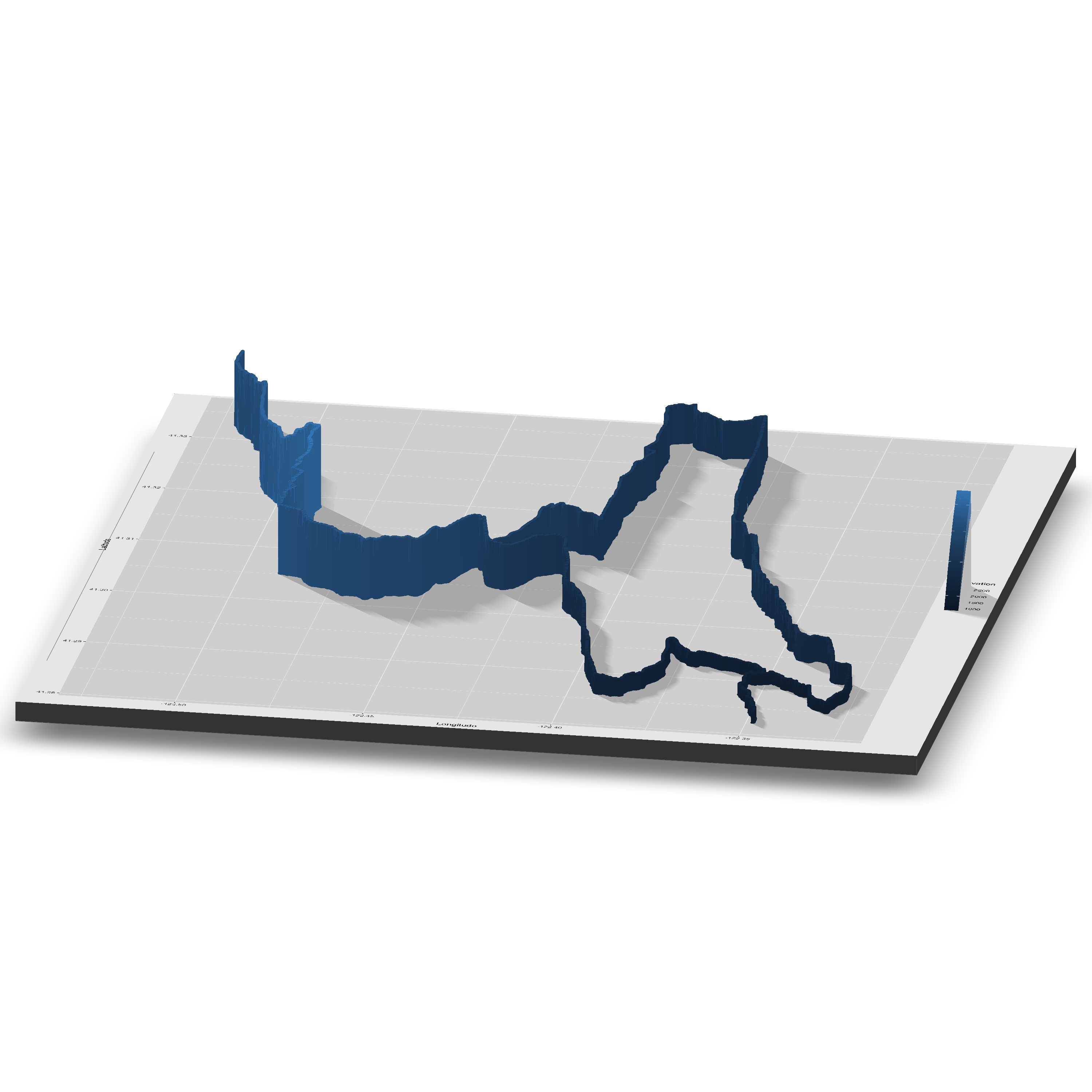
The rayshader package is really cool. You can take ggplot2 figures and make them 3D with this package. The code for doing so is below, but is not run to keep the website rendering time short. It takes a few minutes to render the snapshot view on my Macbook Pro using a few available cores.
TR_p4 <- ggplot() +
          geom_point(data = TrailRun1, aes(x = Longitude, y = Latitude, color = Elevation), size = 2) +
          scale_color_continuous(limits=c(800,2800))
TR_p4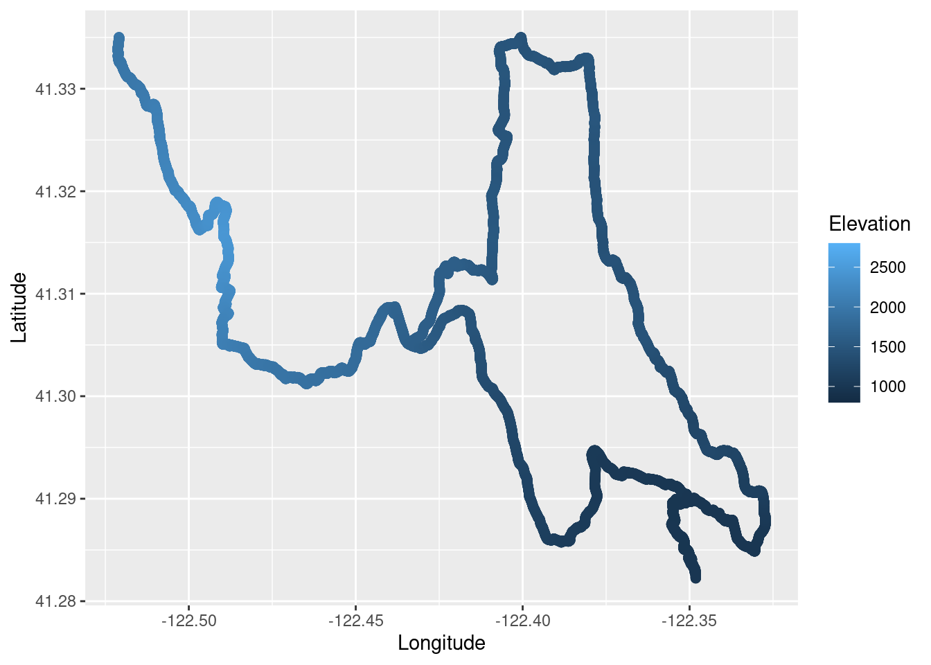
# Not run for website rendering purposes, but you should!
# plot_gg(TR_p4, width = 15, height = 15, multicore = TRUE, scale = 1000,
#         zoom = .7, theta = 10, phi = 20, windowsize = c(3000, 3000))
# Sys.sleep(0.2)
# render_snapshot(filename = "run-elevation-plot3.png", clear = TRUE)