library(sf)
library(tidyverse)
library(rgdal)

setwd("~/DATA/data/calfire.nosync/")
fire <- st_read("fire20_1.gdb")
reserves <- st_read("UC_NRS.gdb")

# subset fire data for 2020
fire2020 <- fire[fire$YEAR_ == "2020",]
plot(fire2020$Shape)
plot(reserves$Shape)
str(fire2020)
str(reserves)A short post overlaying a few different GIS layers on one another for a project we are working on. The databases used are large so I just show the code here with one final image instead of including them in the website repository. I needed to subset the fire perimeters from the Cal Fire database and overlap them with the UC Reserve perimeters. I also needed to in-file some GPS coordinates of post fire sampling sites. I share the code below, but not the data as this project is still in progress. However, the raw data is available:
Intersect the reserves and 2020 fires.
overlaps2020 <-  lengths(st_intersects(fire2020, reserves)) > 0
fire_reserves2020 <- fire2020[overlaps2020,]
plot(fire_reserves2020$Shape, col="orange")
plot(reserves$Shape, col="blue", add = TRUE)
Take a look at the names of the fires that overlap and then specifically subset them for later processing.
fire_reserves2020$FIRE_NAME
river_fire <- subset(fire2020, FIRE_NAME == "RIVER")
scu_complex_fire <- subset(fire2020, FIRE_NAME == "SCU COMPLEX")
hennessey_fire <- subset(fire2020, FIRE_NAME == "HENNESSEY")
dolan_fire <- subset(fire2020, FIRE_NAME == "DOLAN")
snow_fire <- subset(fire2020, FIRE_NAME == "SNOW") # did not collect field data here
Infile the arthropod sampling locations and make a coordinates dataframe.
setwd("~/DATA/data/")
arthro_data <- read_csv("Post-FireMonitoring_Arthropod_SamplingLocations.csv")
arthro_coords <- data.frame(x = arthro_data$LONGITUDE, y = arthro_data$LATITUDE)
I converted the data frame to a spatial object with the appropriate map projection information. This then allowed me to convert Lat/Long coordinates to the same projection that the Cal Fire and UC Reserve System perimeters data are projected in (California Albers- EPSG:3310).
# make spatial dataframe with lat long coords using the RGDAL package functions
coordinates(arthro_coords) <- ~x+y
proj4string(arthro_coords) <- CRS("+proj=longlat +datum=WGS84")
str(arthro_coords)
arthro_3310 <- spTransform(df, CRS("+init=epsg:3310"))
arthro_3310
str(arthro_3310)
# double check with plot
plot(reserves$Shape, col="blue")
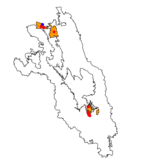
plot(arthro_3310, , col = "red", add = TRUE)Convert the object to and sf object for quick plotting. Calculate the overlays between the fire sampling site and the control sampling sites. Overlay the fire perimeter, the reserve perimeters, and the sampling sites. To make it more clear I chose the Hennessey Fire which burned across two reserve boundaries in 2020.
# convert to sf package object
fire_pts2 <- st_as_sf(arthro_3310)
str(fire_pts2)

# overlay points and fire shapes
fire_yes = lengths(st_intersects(fire_pts2, hennessey_fire)) > 0
fire_yes

# layer all the plots
plot(hennessey_fire$Shape) # fire shape
plot(reserves$Shape, col="orange", add=TRUE) # local reserves shape
plot(fire_pts2, pch=19, col="blue", add=TRUE); # all samples
plot(fire_pts2[fire_yes,], pch=19, col="red", add=TRUE); # samples in fire
It is over-plotted in this view, but this demonstrates the idea. The Hennessey fire perimeter is shown in black, reserves in orange, reserve sampling sites within the fire perimeter in red, and sampling sites within the reserve, but outside the fire perimeter in blue.