Cody Markelz - Mount Shasta Wilderness Wildflowers

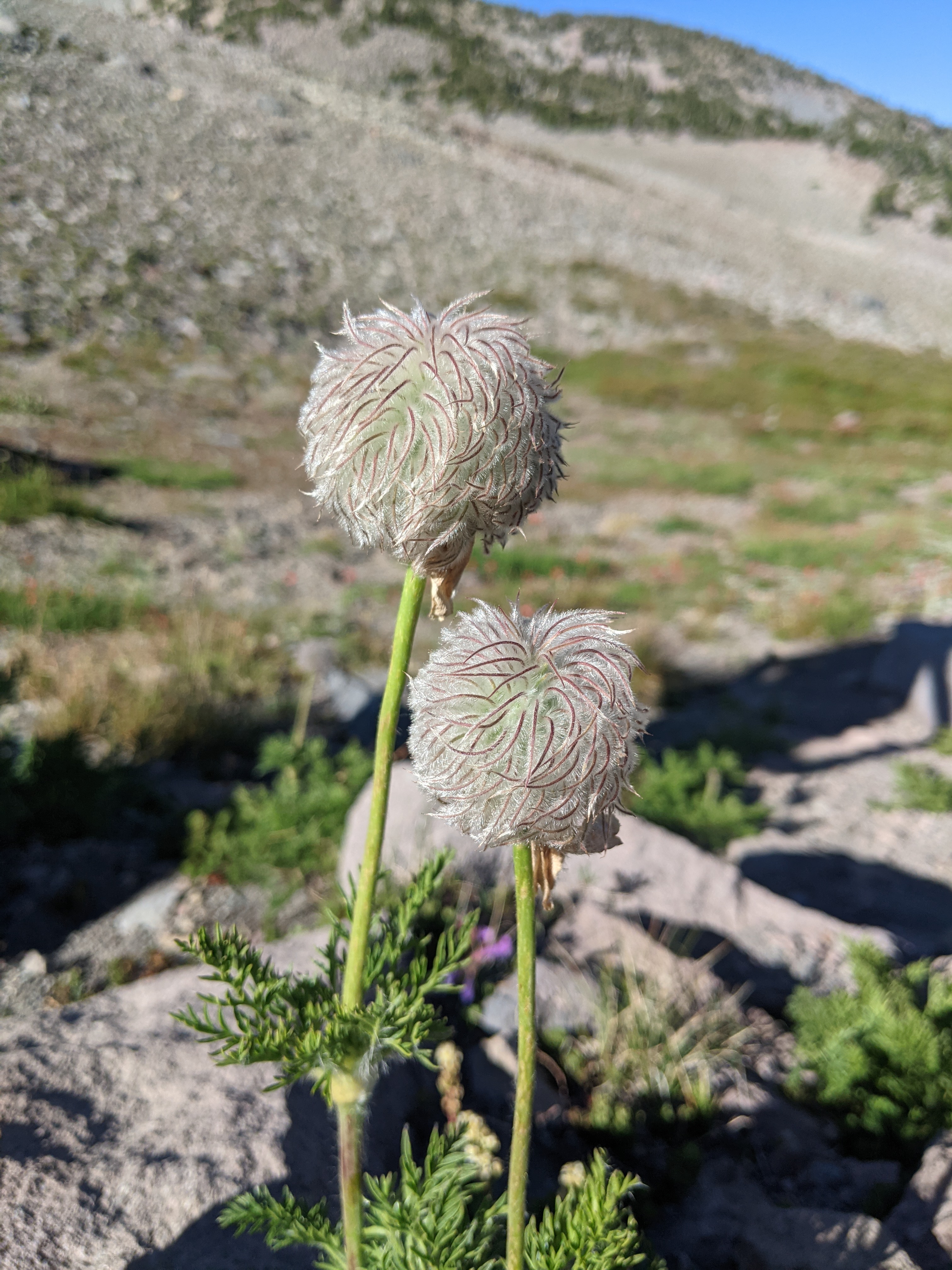
I went on a quick overnight to a spring fed creek above 8000 feet on Mount Shasta. I noticed these interesting flowers that I have never seen before. They reminded me of something that Dr. Seuss would have illustrated in his various children’s books. After searching the internet with no luck I finally needed rely on some California Botany experts to help with the ID: Anemone occidentalis. The hair-like calyx tissue on top of each ovary are what give this plant it’s unique look once reproductively mature. These are similar structures to white dandelion heads and aid in seed dispersal via wind.

Load the libraries.

library(tidyverse)
library(rgbif)
library(gpx)

Make the large Northern California polygon to look for observations in GBIF.

norcal_geometry <- paste('POLYGON((-124.4323 42.0021, -121.5045 42.0021, -121.5045 40.194, -124.4323 40.194, -124.4323 42.0021))')

dr_seuss <- occ_data(scientificName = "Anemone occidentalis", hasCoordinate = TRUE, limit = 1000,
                   geometry = norcal_geometry)
# length(dr_seuss)
head(dr_seuss)

$meta
$meta$offset
[1] 0

$meta$limit
[1] 300

$meta$endOfRecords
[1] TRUE

$meta$count
[1] 44


$data
# A tibble: 44 × 114
   key    scien…¹ decim…² decim…³ issues datas…⁴ publi…⁵ insta…⁶ publi…⁷ proto…⁸
   <chr>  <chr>     <dbl>   <dbl> <chr>  <chr>   <chr>   <chr>   <chr>   <chr>  
 1 40229… Anemon…    41.4   -122. cdc    b05154… a8a2b5… cb27a4… US      DWC_AR…
 2 40229… Anemon…    41.4   -122. cdc    b05154… a8a2b5… cb27a4… US      DWC_AR…
 3 40229… Anemon…    41.4   -122. cdc    b05154… a8a2b5… cb27a4… US      DWC_AR…
 4 89974… Anemon…    41.6   -123. cdc,c… 7a2660… 0674ae… 6038e5… DE      BIOCASE
 5 24179… Anemon…    40.5   -122. cdc,a… ae33dc… c6e100… cb27a4… US      DWC_AR…
 6 29820… Anemon…    41.2   -123. cdc,c… 695862… c10e9f… cb27a4… US      DWC_AR…
 7 33207… Anemon…    41.5   -122. cdc,g… 677aec… 314e47… cb27a4… US      DWC_AR…
 8 33207… Anemon…    41.2   -123. cdc,g… 677aec… 314e47… cb27a4… US      DWC_AR…
 9 33207… Anemon…    41.5   -123. cdc,g… 677aec… 314e47… cb27a4… US      DWC_AR…
10 29820… Anemon…    41.6   -123. cdc,g… 695862… c10e9f… cb27a4… US      DWC_AR…
# … with 34 more rows, 104 more variables: lastCrawled <chr>, lastParsed <chr>,
#   crawlId <int>, hostingOrganizationKey <chr>, basisOfRecord <chr>,
#   occurrenceStatus <chr>, taxonKey <int>, kingdomKey <int>, phylumKey <int>,
#   classKey <int>, orderKey <int>, familyKey <int>, genusKey <int>,
#   speciesKey <int>, acceptedTaxonKey <int>, acceptedScientificName <chr>,
#   kingdom <chr>, phylum <chr>, order <chr>, family <chr>, genus <chr>,
#   species <chr>, genericName <chr>, specificEpithet <chr>, taxonRank <chr>, …

Quick map of observations in Northern California. There are a few observations across the general bioregion I live near, but none on the hike I went on.

dr_seuss_coords <- dr_seuss$data[ , c("decimalLongitude", "decimalLatitude", "occurrenceStatus", "coordinateUncertaintyInMeters", "institutionCode", "references")]

maps::map(database = "state", region = "california")
points(dr_seuss_coords[ , c("decimalLongitude", "decimalLatitude")], pch = ".", col = "red", cex = 3)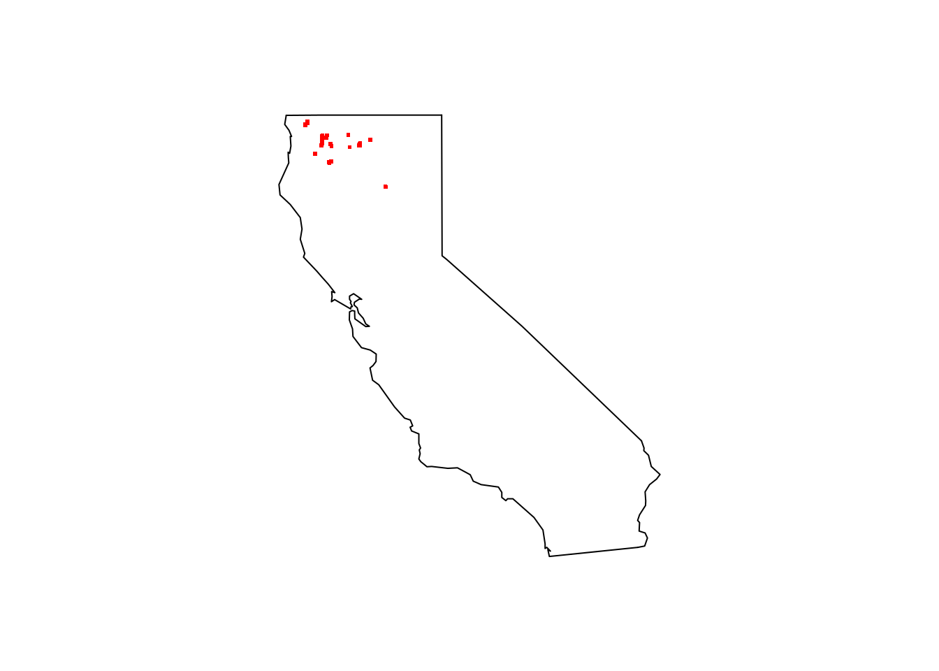

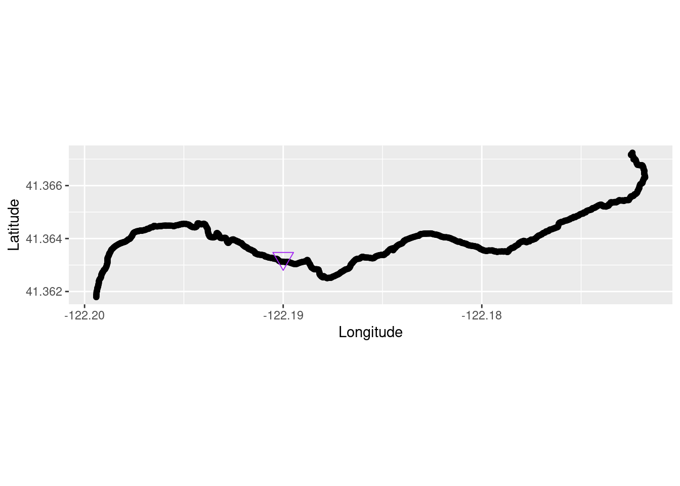
Pull in my hike data using the gpx R library and subset the route to make plotting easier.

hike <-  read_gpx('~/DATA/data/mount_shasta_hiking.gpx')
hike1 <- as.data.frame(hike$routes)

Overlay the hiking data and the image/observation coordinates as a triangle.

hike_plot2 <- ggplot() +
          coord_quickmap() +
          geom_point(data = hike1, aes(x = Longitude, y = Latitude), color = 'black') +
          geom_point(aes(x = -122.19, y = 41.36325), pch=25, size= 5, colour="purple") +
          xlab("Longitude") + ylab("Latitude")
hike_plot2