library(rgbif)
library(sf)
library(tidyverse)
library(rnaturalearth)
library(rnaturalearthdata)
Introduction
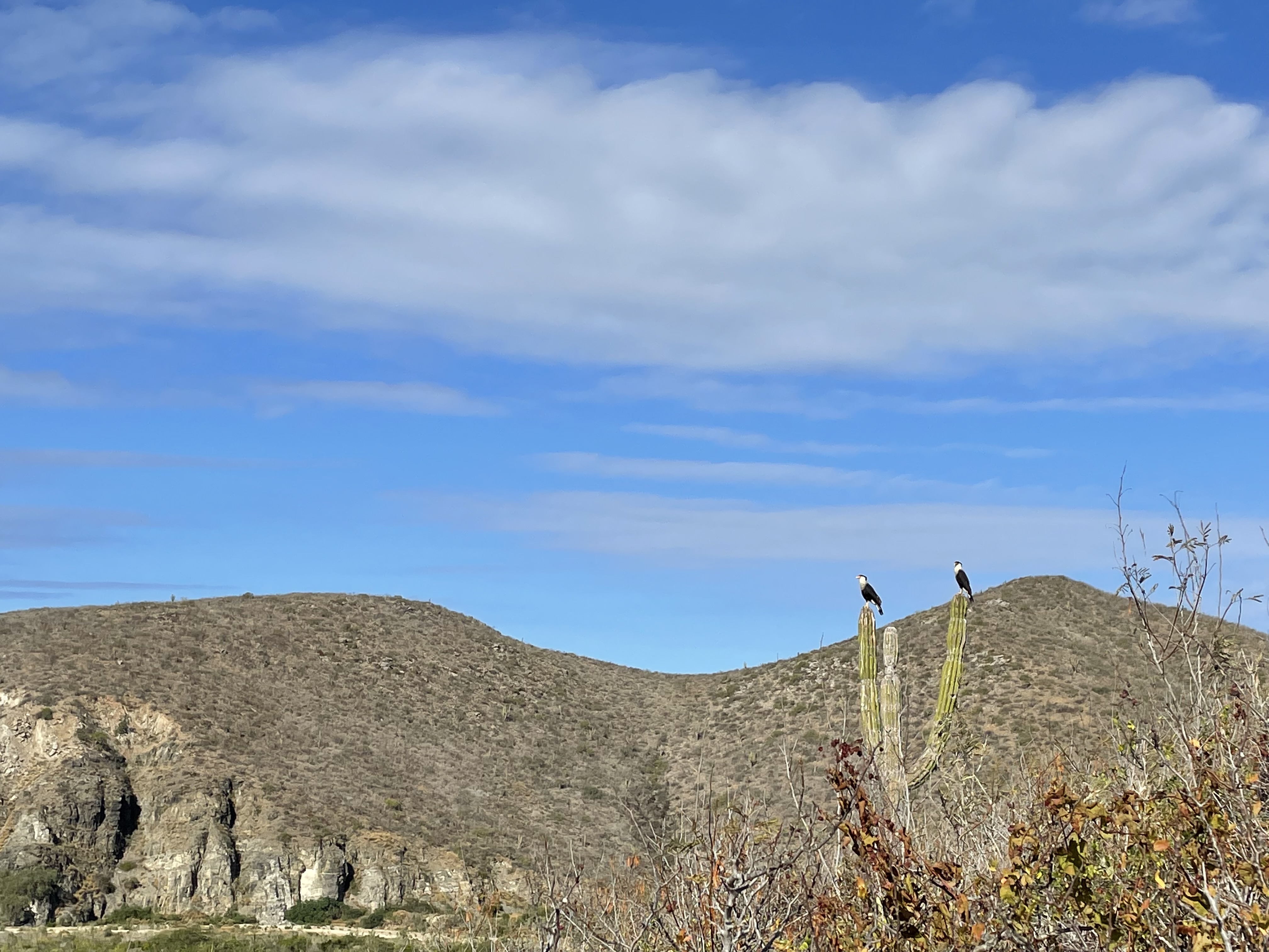
I saw these beautiful birds while out train running in Baja Sur, Mexico. I had never even heard of them until now, but Crested Caracaras are really interesting birds! They are technically falcons, but act more like buzzards. This might explain why they were looking over me while I exercised in the desert. I saw the distribution map on the wikipedia link, but I wanted to see how many entries in GBIF there were in the general region I was visiting.
Load the libraries
Subset our search to only Southern Baja Sur. I used this website to make a quick bounding box which I convert into a polygon as an input to the GBIF search function. I search the general area and then clean up the output for easier plotting.
baja_geometry <- paste('POLYGON((-112.632285206 22.4136232805, -109.1001807138 22.4136232805, -109.1001807138 25.4259663625, -112.632285206 25.4259663625, -112.632285206 22.4136232805))')

caracara <- occ_data(scientificName = "Caracara plancus", hasCoordinate = TRUE, limit = 10000,
                     geometry = baja_geometry )

caracara_coords <- caracara$data[ , c("decimalLongitude", "decimalLatitude",
 "individualCount", "occurrenceStatus", "coordinateUncertaintyInMeters",
  "institutionCode", "references")]
The standard maps packages I use did not have a good map of the Mexican states for quick plotting and that also integrate with the sf package well. rnaturalearth and rnaturalearthdata are good resources for plotting specific regions in various countries using the maps stored as sf objects. I subset the larger dataset to just zoom in on Mexico and plot the appoximate location where my observation was.
caracara_obs <- data.frame(decimalLongitude = c(-110.18917658541324), decimalLatitude = c(23.369598786877447))

world_maps <- ne_countries(scale = "medium", returnclass = "sf")
mexico <- subset(world_maps, name == "Mexico")

ggplot(data = mexico) +
                geom_sf() +
                geom_point(data = caracara_obs, aes(x = decimalLongitude, y = decimalLatitude), color = 'red')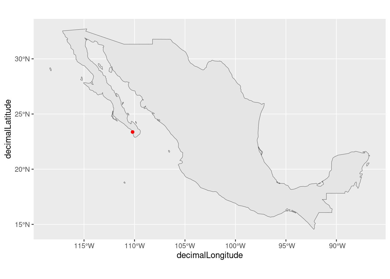
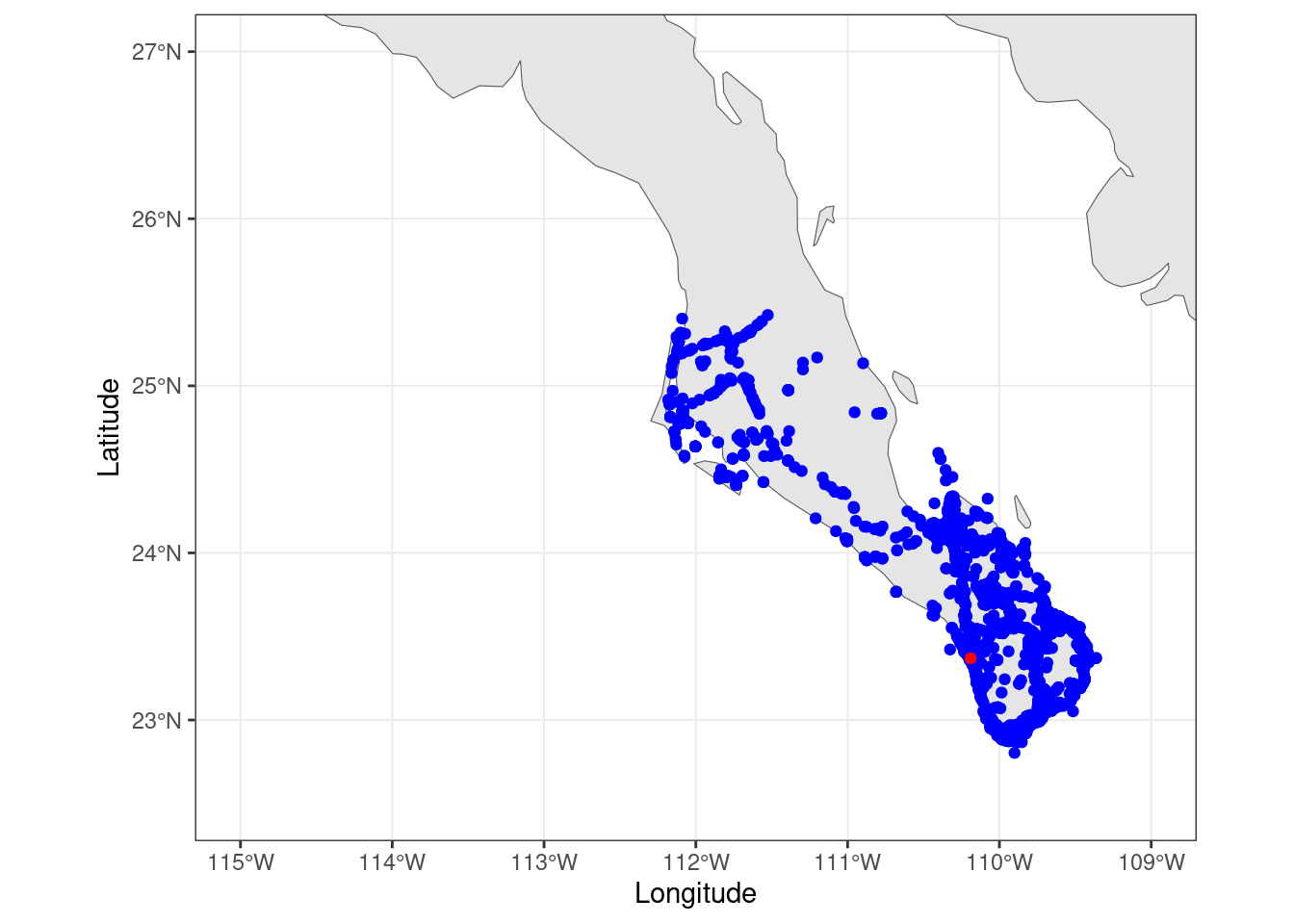
Zoom into the Baja penninsula and plot all the points. There have been many observations of the Crested Caracara all over the general region I visited.
theme_set(theme_bw())
ggplot(data = mexico) +
        geom_sf() +
        geom_point(data = caracara_coords, aes(x = decimalLongitude, y = decimalLatitude), color = 'blue') +
        geom_point(data = caracara_obs, aes(x = decimalLongitude, y = decimalLatitude), color = 'red')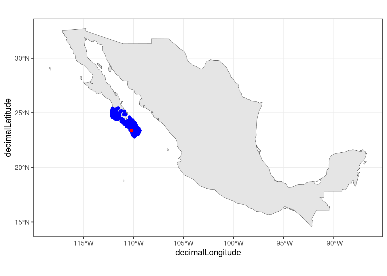
ggplot(data = mexico) +
        geom_sf() +
        geom_point(data = caracara_coords, aes(x = decimalLongitude, y = decimalLatitude), color = 'blue') +
        geom_point(data = caracara_obs, aes(x = decimalLongitude, y = decimalLatitude), color = 'red') +
        coord_sf(xlim = c(-115, -109), ylim = c(22.5, 27), expand = TRUE) +
        xlab("Longitude") + ylab("Latitude")