library(rgbif)
library(sf)
library(tidyverse)
library(rnaturalearth)
library(rnaturalearthdata)
Introduction
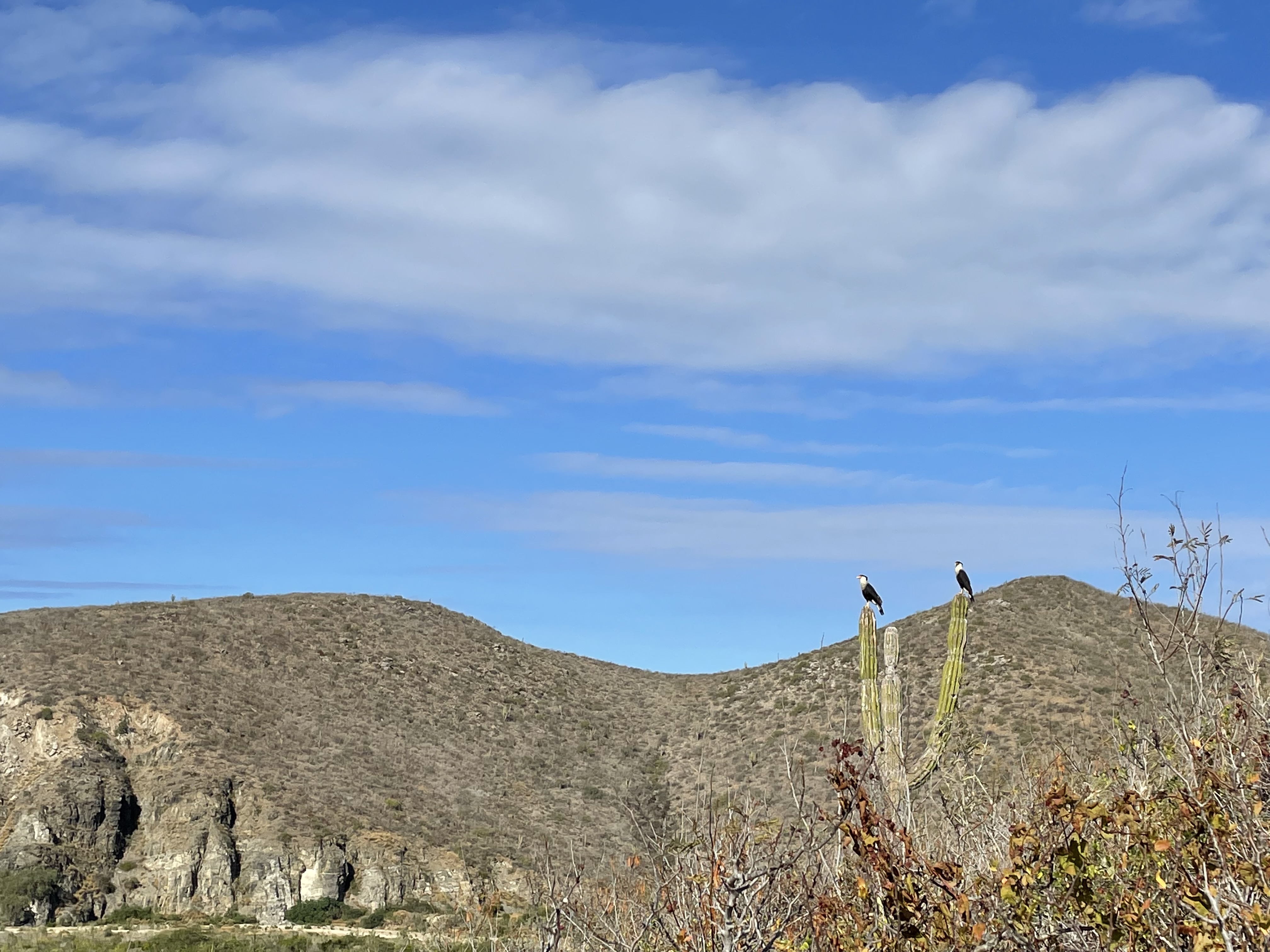
The Crested caracara’s I talked about in my last post are sitting on top of a Giant Cardon Cacti (Pachycereus pringlei). I wanted to take a look to see if the cacti were as widely distributed in the area as the Caracaras.
Load the libraries
Subset our search to only Southern Baja Sur.
baja_geometry <- paste('POLYGON((-112.632285206 22.4136232805, -109.1001807138 22.4136232805, -109.1001807138 25.4259663625, -112.632285206 25.4259663625, -112.632285206 22.4136232805))')

cacti <- occ_data(scientificName = "Pachycereus pringlei", hasCoordinate = TRUE, limit = 10000,
                     geometry = baja_geometry )

cacti_coords <- cacti$data[ , c("decimalLongitude", "decimalLatitude",
 "individualCount", "occurrenceStatus", "coordinateUncertaintyInMeters",
  "institutionCode", "references")]
I subset the larger dataset to just zoom in on Mexico and plot the appoximate location where my observation was.
cacti_obs <- data.frame(decimalLongitude = c(-110.18917658541324), decimalLatitude = c(23.369598786877447))

world_maps <- ne_countries(scale = "medium", returnclass = "sf")
mexico <- subset(world_maps, name == "Mexico")

ggplot(data = mexico) +
                geom_sf() +
                geom_point(data = cacti_obs, aes(x = decimalLongitude, y = decimalLatitude), color = 'red')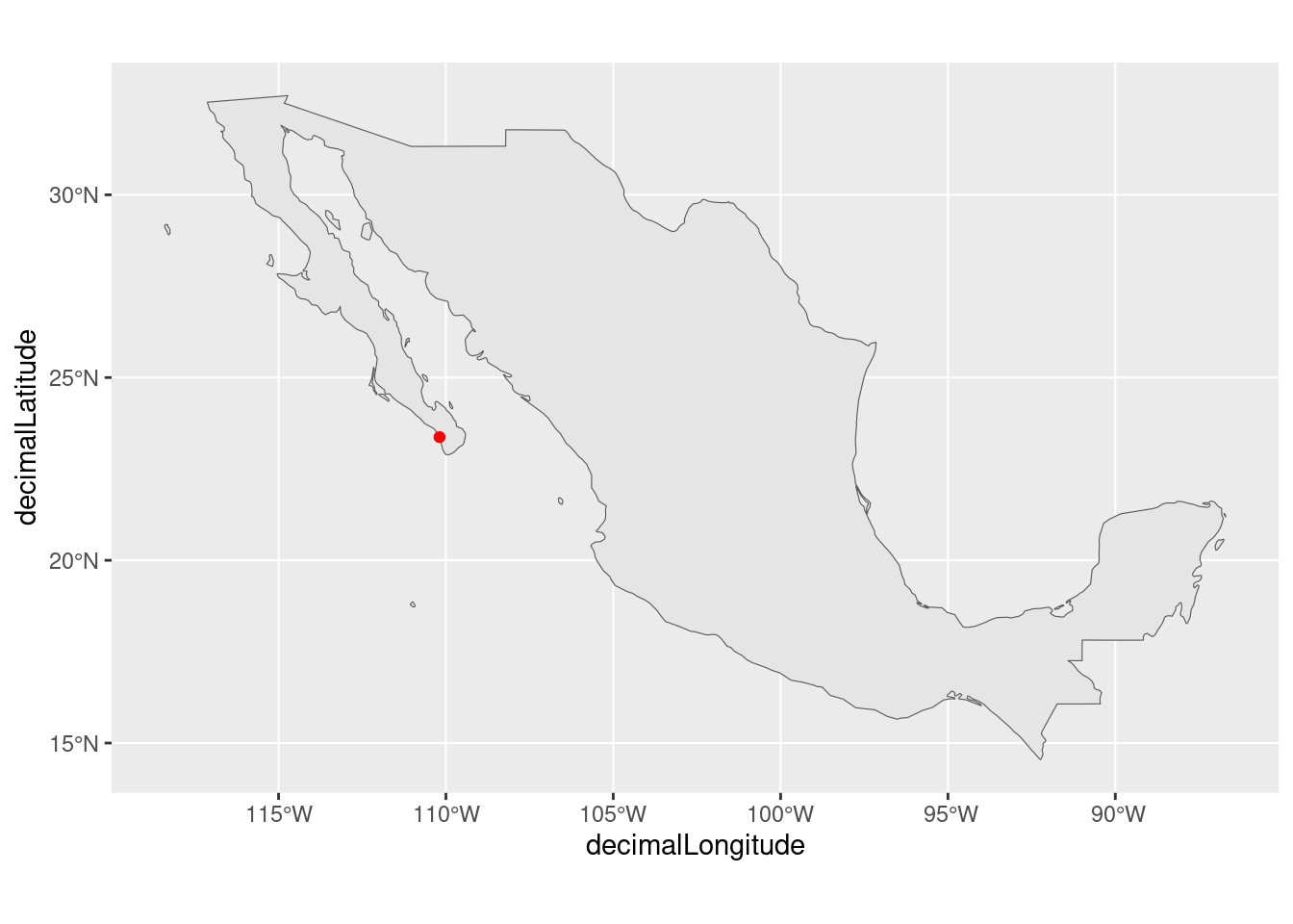
Zoom into the Baja penninsula and plot all the points. There have been many observations of both the Giant Cardon Cacti and the Crested caracara all over the general region I visited.
theme_set(theme_bw())
ggplot(data = mexico) +
        geom_sf() +
        geom_point(data = cacti_coords, aes(x = decimalLongitude, y = decimalLatitude), color = 'blue') +
        geom_point(data = cacti_obs, aes(x = decimalLongitude, y = decimalLatitude), color = 'red')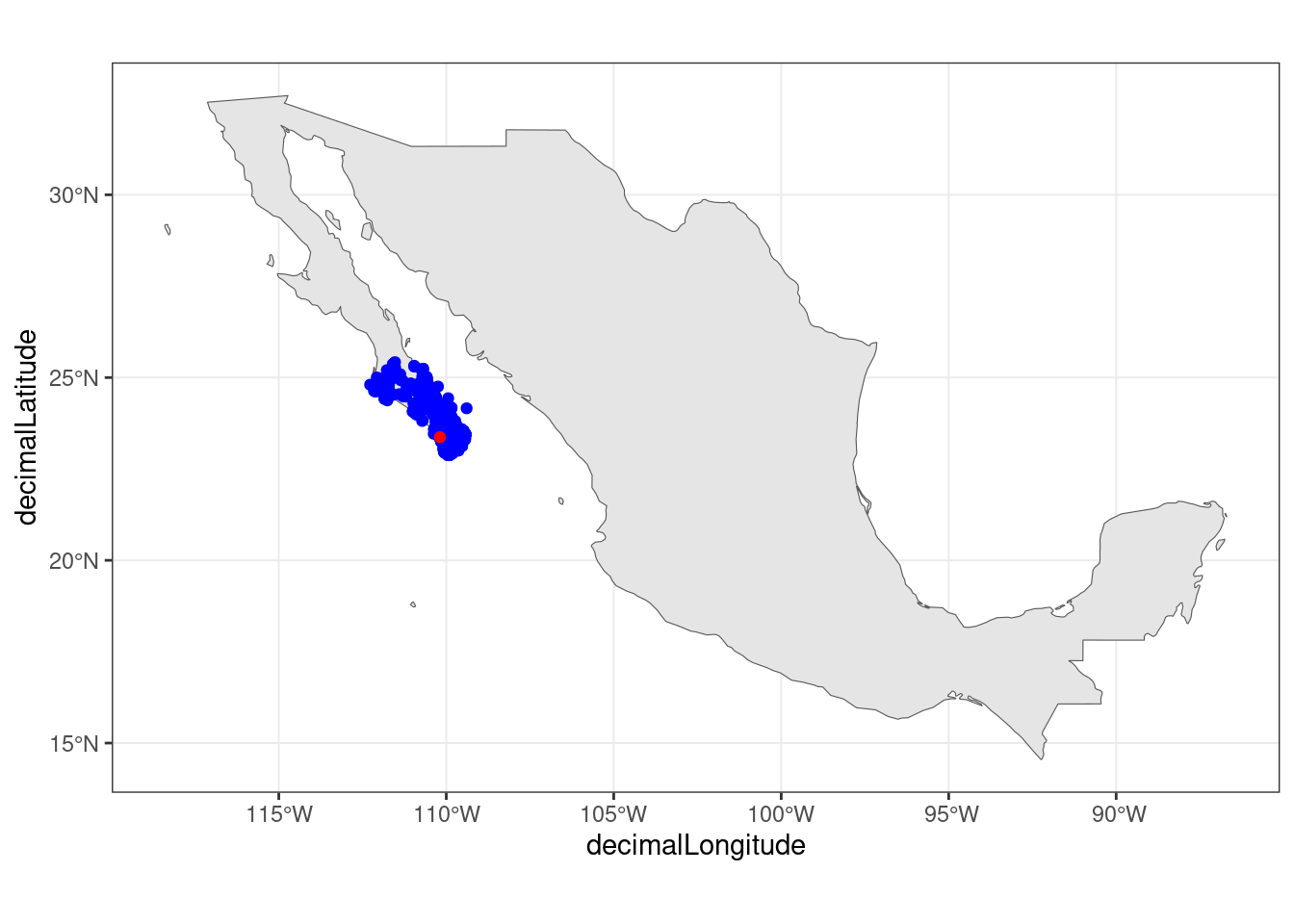
ggplot(data = mexico) +
        geom_sf() +
        geom_point(data = cacti_coords, aes(x = decimalLongitude, y = decimalLatitude), color = 'blue') +
        geom_point(data = cacti_obs, aes(x = decimalLongitude, y = decimalLatitude), color = 'red') +
        coord_sf(xlim = c(-115, -109), ylim = c(22.5, 27), expand = TRUE) +
        xlab("Longitude") + ylab("Latitude")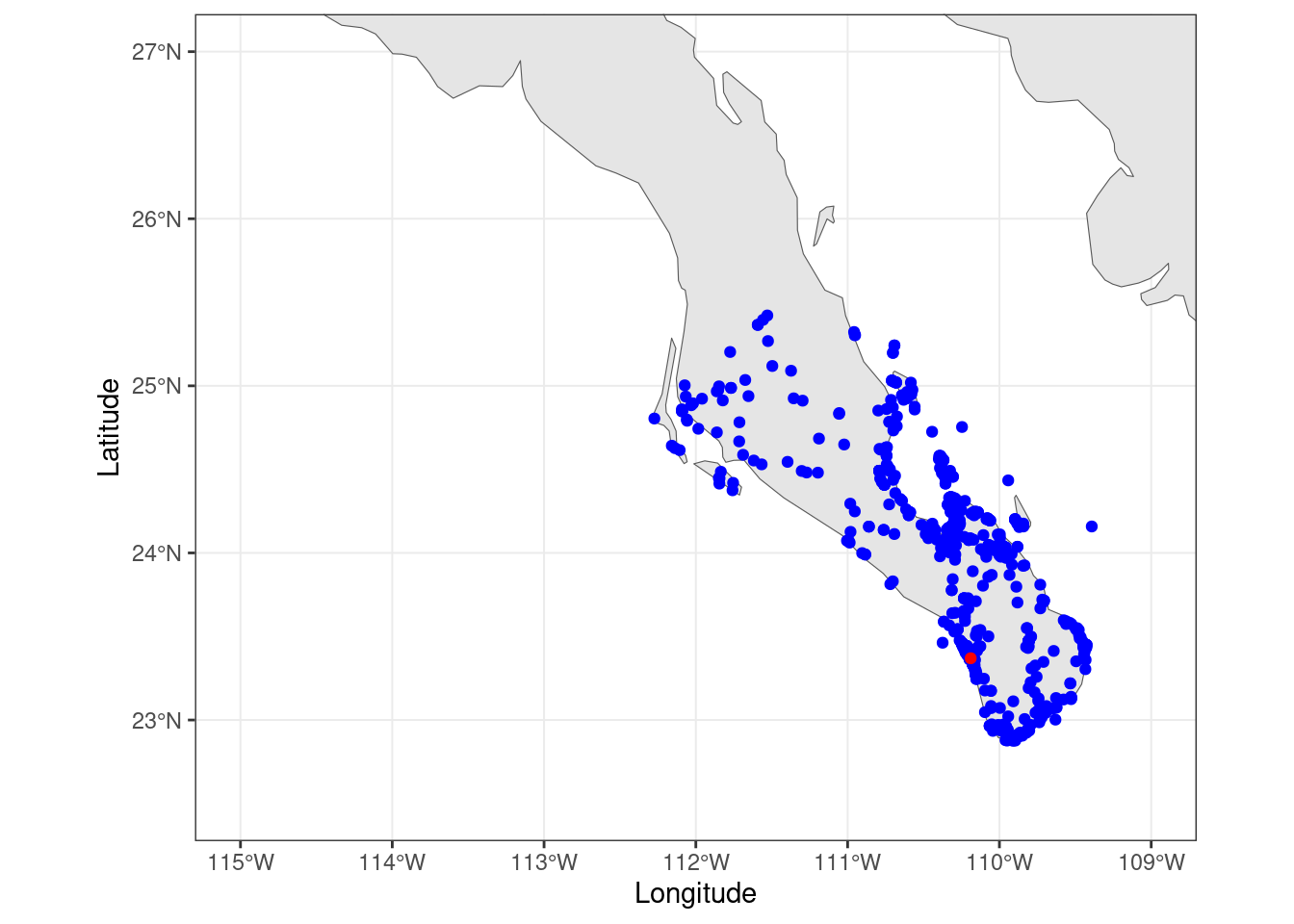
ggsave("~/DATA/images/cardon-cacti-map.png")